Alignment methods benchmark (template-based ROI case)

In this tutorial, we compare various methods of alignment on a pairwise alignment problem for Individual Brain Charting subjects. For each subject, we have a lot of functional informations in the form of several task-based contrast per subject. We will just work here on a ROI.

We mostly rely on python common packages and on nilearn to handle functional data in a clean fashion.

To run this example, you must launch IPython via ipython --matplotlib in a terminal, or use jupyter-notebook.

Retrieve the data

In this example we use the IBC dataset, which include a large number of different contrasts maps for 12 subjects.

The contrasts come from tasks in the Archi and HCP fMRI batteries, designed to probe a range of cognitive functions, including:

• Motor control: finger, foot, and tongue movements

• Social cognition: interpreting short films and stories

• Spatial orientation: judging orientation and hand-side

• Numerical reasoning: reading and listening to math problems

• Emotion processing: judging facial expressions

• Reward processing: responding to gains and losses

• Working memory: maintaining sequences of faces and objects

• Object categorization: matching and comparing visual stimuli

# We download the images for subjects sub-01 and sub-02.
# ``files`` is the list of paths for each subjects.
# ``df`` is a dataframe with metadata about each of them.
# ``mask`` is the common mask for IBC subjects.

from fmralign.fetch_example_data import fetch_ibc_subjects_contrasts

sub_ids = ["sub-01", "sub-02", "sub-04"]
files, df, mask = fetch_ibc_subjects_contrasts(sub_ids)

[get_dataset_dir] Dataset found in /home/runner/nilearn_data/ibc

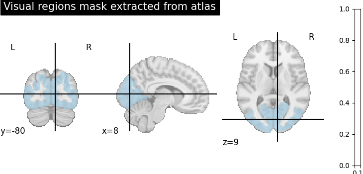
Extract a mask for the visual cortex from Yeo Atlas

First, we fetch and plot the complete atlas

from nilearn import datasets, plotting
from nilearn.image import concat_imgs, load_img, new_img_like, resample_to_img

atlas_yeo_2011 = datasets.fetch_atlas_yeo_2011()
atlas = load_img(atlas_yeo_2011.thick_7)

# Select visual cortex, create a mask and resample it to the right resolution

mask_visual = new_img_like(atlas, atlas.get_fdata() == 1)
resampled_mask_visual = resample_to_img(
    mask_visual, mask, interpolation="nearest"
)

# Plot the mask we will use
plotting.plot_roi(
    resampled_mask_visual,
    title="Visual regions mask extracted from atlas",
    cut_coords=(8, -80, 9),
    colorbar=False,
    cmap="Paired",
)

/home/runner/work/fmralign/fmralign/examples/plot_alignment_methods_benchmark.py:55: DeprecationWarning: From release >=0.13.0, instead of returning several atlas image accessible via different keys, this fetcher will return the atlas as a dictionary with a single atlas image, accessible through a 'maps' key. To suppress this warning, Please use the parameters 'n_networks' and 'thickness' to specify the exact atlas image you want.
  atlas_yeo_2011 = datasets.fetch_atlas_yeo_2011()
[fetch_atlas_yeo_2011] Dataset found in /home/runner/nilearn_data/yeo_2011
/home/runner/work/fmralign/fmralign/examples/plot_alignment_methods_benchmark.py:61: FutureWarning: 'force_resample' will be set to 'True' by default in Nilearn 0.13.0.
Use 'force_resample=True' to suppress this warning.
  resampled_mask_visual = resample_to_img(
/home/runner/work/fmralign/fmralign/examples/plot_alignment_methods_benchmark.py:61: FutureWarning: From release 0.13.0 onwards, this function will, by default, copy the header of the input image to the output. Currently, the header is reset to the default Nifti1Header. To suppress this warning and use the new behavior, set `copy_header=True`.
  resampled_mask_visual = resample_to_img(

<nilearn.plotting.displays._slicers.OrthoSlicer object at 0x7f1c2fe0c9b0>

Define a masker

We define a nilearn masker that will be used to handle relevant data. For more information, visit : ‘http://nilearn.github.io/manipulating_images/masker_objects.html’

from nilearn.maskers import NiftiMasker

roi_masker = NiftiMasker(mask_img=resampled_mask_visual).fit()

Prepare the data

For each subject, for each task and conditions, our dataset contains two independent acquisitions, similar except for one acquisition parameter, the encoding phase used that was either Antero-Posterior (AP) or Postero-Anterior (PA). Although this induces small differences in the final data, we will take advantage of these pseudo-duplicates to define training and test samples.

# The training set:
# * source_train: AP acquisitions from source subjects (sub-01, sub-02).
# * target_train: AP acquisitions from the target subject (sub-04).
#

source_subjects = [sub for sub in sub_ids if sub != "sub-04"]
source_train = [
    concat_imgs(df[(df.subject == sub) & (df.acquisition == "ap")].path.values)
    for sub in source_subjects
]
target_train = concat_imgs(
    df[(df.subject == "sub-04") & (df.acquisition == "ap")].path.values
)

# The testing set:
# * source_test: PA acquisitions from source subjects (sub-01, sub-02).
# * target test: PA acquisitions from the target subject (sub-04).
#

source_test = [
    concat_imgs(df[(df.subject == sub) & (df.acquisition == "pa")].path.values)
    for sub in source_subjects
]
target_test = concat_imgs(
    df[(df.subject == "sub-04") & (df.acquisition == "pa")].path.values
)

Choose the number of regions for local alignment

First, as we will proceed to local alignment we choose a suitable number of regions so that each of them is approximately 100 voxels wide. Then our estimator will first make a functional clustering of voxels based on train data to divide them into meaningful regions.

import numpy as np

n_voxels = roi_masker.mask_img_.get_fdata().sum()
print(f"The chosen region of interest contains {n_voxels} voxels")
n_pieces = int(np.round(n_voxels / 100))
print(f"We will cluster them in {n_pieces} regions")

The chosen region of interest contains 6631.0 voxels
We will cluster them in 66 regions

Define the estimators, fit them and do a prediction

On each region, we search for a transformation R that is either :

• orthogonal, i.e. R orthogonal, scaling sc s.t. ||sc RX - Y ||^2 is minimized

• the optimal transport plan, which yields the minimal transport cost while respecting the mass conservation constraints. Calculated with entropic regularization.

• the shared response model (SRM), which computes a shared response space from different subjects, and then projects individual subject data into it.

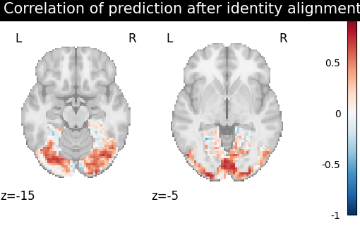
Then for each method we define the estimator, fit it, predict the new image and plot its correlation with the real signal.

Fit and score the Orthogonal and Optimal Transport estimators

from fmralign.metrics import score_voxelwise
from fmralign.template_alignment import TemplateAlignment

methods = ["scaled_orthogonal", "optimal_transport"]

# Prepare to store the results
titles, aligned_scores = [], []

for i, method in enumerate(methods):
    alignment_estimator = TemplateAlignment(
        alignment_method=method, n_pieces=n_pieces, masker=roi_masker
    )
    alignment_estimator.fit(source_train)
    target_pred = alignment_estimator.transform(target_train)

    # derive correlation between prediction, test
    method_error = score_voxelwise(
        target_test, target_pred, masker=roi_masker, loss="corr"
    )

    # store the results for plotting later
    aligned_score = roi_masker.inverse_transform(method_error)
    titles.append(f"Correlation of prediction after {method} alignment")
    aligned_scores.append(aligned_score)

/home/runner/work/fmralign/fmralign/fmralign/_utils.py:258: UserWarning: Overriding provided-default estimator parameters with provided masker parameters :
Parameter mask_strategy :
    Masker parameter background - overriding estimator parameter epi
Parameter smoothing_fwhm :
    Masker parameter None - overriding estimator parameter 4.0

  parcellation.fit(images_to_parcel)
[TemplateAlignment.fit] Resampling mask
/home/runner/work/fmralign/fmralign/.venv/lib/python3.12/site-packages/sklearn/cluster/_agglomerative.py:321: UserWarning: the number of connected components of the connectivity matrix is 11 > 1. Completing it to avoid stopping the tree early.
  connectivity, n_connected_components = _fix_connectivity(
/home/runner/work/fmralign/fmralign/.venv/lib/python3.12/site-packages/joblib/memory.py:326: UserWarning: Data array used to create a new image contains 64-bit ints. This is likely due to creating the array with numpy and passing `int` as the `dtype`. Many tools such as FSL and SPM cannot deal with int64 in Nifti images, so for compatibility the data has been converted to int32.
  return self.func(*args, **kwargs)
/home/runner/work/fmralign/fmralign/fmralign/metrics.py:62: ConstantInputWarning: An input array is constant; the correlation coefficient is not defined.
  pearsonr(X_gt[:, vox], X_pred[:, vox])[
/home/runner/work/fmralign/fmralign/fmralign/_utils.py:258: UserWarning: Overriding provided-default estimator parameters with provided masker parameters :
Parameter mask_strategy :
    Masker parameter background - overriding estimator parameter epi
Parameter smoothing_fwhm :
    Masker parameter None - overriding estimator parameter 4.0

  parcellation.fit(images_to_parcel)
[TemplateAlignment.fit] Resampling mask
/home/runner/work/fmralign/fmralign/.venv/lib/python3.12/site-packages/sklearn/cluster/_agglomerative.py:321: UserWarning: the number of connected components of the connectivity matrix is 11 > 1. Completing it to avoid stopping the tree early.
  connectivity, n_connected_components = _fix_connectivity(
/home/runner/work/fmralign/fmralign/.venv/lib/python3.12/site-packages/joblib/memory.py:326: UserWarning: Data array used to create a new image contains 64-bit ints. This is likely due to creating the array with numpy and passing `int` as the `dtype`. Many tools such as FSL and SPM cannot deal with int64 in Nifti images, so for compatibility the data has been converted to int32.
  return self.func(*args, **kwargs)
/home/runner/work/fmralign/fmralign/fmralign/metrics.py:62: ConstantInputWarning: An input array is constant; the correlation coefficient is not defined.
  pearsonr(X_gt[:, vox], X_pred[:, vox])[

Fit and score the SRM estimator

# The IdentifiableFastSRM version of SRM ensures that the solution is unique.
from fastsrm.identifiable_srm import IdentifiableFastSRM

srm = IdentifiableFastSRM(
    n_components=30,
    n_iter=10,
)

# Step 1: Fit SRM on training data from source subjects
shared_response = srm.fit_transform(
    [roi_masker.transform(s).T for s in source_train]
)

# Step 2: Freeze the SRM model and add target subject data. This projects the
# target subject data into the shared response space.
srm.aggregate = None
srm.add_subjects([roi_masker.transform(target_train).T], shared_response)

# Step 3: Use SRM to transform new test data from the target subject
aligned_test = srm.transform([roi_masker.transform(target_test).T])
aligned_pred = roi_masker.inverse_transform(
    srm.inverse_transform(aligned_test[0])[0].T
)

# Step 4: Evaluate voxelwise correlation between predicted and true test
# signals. Store the results for plotting later.
srm_error = score_voxelwise(
    target_test, aligned_pred, masker=roi_masker, loss="corr"
)
srm_score = roi_masker.inverse_transform(srm_error)
titles.append("Correlation of prediction after SRM alignment")
aligned_scores.append(srm_score)

ProbSRM did not converge. Current diff is 23.758430

Plot the results

import matplotlib.pyplot as plt

fig, axes = plt.subplots(3, 1, figsize=(8, 12))

for i, (score, title) in enumerate(zip(aligned_scores, titles)):
    plotting.plot_stat_map(
        score,
        display_mode="z",
        cut_coords=[-15, -5],
        vmax=1,
        title=title,
        axes=axes[i],
        colorbar=True,
    )

plt.show()

/home/runner/work/fmralign/fmralign/examples/plot_alignment_methods_benchmark.py:223: UserWarning: Non-finite values detected. These values will be replaced with zeros.
  plotting.plot_stat_map(

Summary:

We compared TemplateAlignment methods (scaled orthogonal, optimal transport) with SRM-based alignment on visual cortex activity. You can see that SRM introduces the most smoothness in the transformation, resulting in higher correlation values.